Top-K Trending System Design

A Top-K Trending System continuously processes user activity and finds the most popular or trending items within a given time window.

For example:

Top 10 hashtags right now
Top 50 most watched videos today
Top 100 songs in the last 7 days
Top topics in India during the last hour

At small scale, the problem looks simple:

Count Events
     ↓
Calculate Item Counts
     ↓
Sort by Count
     ↓
Return Top K

At large scale, repeatedly counting and sorting all events becomes expensive.

A real-time trending system may process millions of events, track millions of items, support different time windows, and still need to return Top-K results within milliseconds.

The main system design problem is:

How do we continuously find the Top-K items from a massive event stream without repeatedly scanning and sorting the complete dataset?

What Is a Top-K Trending System?

A Top-K system finds the K highest-scoring items from a large set.

Suppose users are posting hashtags:

#worldcup
#ai
#systemdesign
#football
#worldcup
#ai
#worldcup

Their counts become:

#worldcup       3
#ai             2
#football       1
#systemdesign   1

For K = 2, the result is:

1. #worldcup
2. #ai

This is the basic Top-K frequent items problem.

A production trending system adds another important factor: time.

For example:

Top 10 hashtags in the last 5 minutes
Top 100 songs in the last 7 days

As time moves forward, old events must stop contributing to the score.

This turns a simple counting problem into a distributed stream-processing and sliding-window problem.

What Does “Trending” Mean?

Before designing the architecture, we need to define what trending means because popularity and trending are not always the same.

Consider:

#football
Historical mentions = 10,000,000
Current rate        = 100/minute

#newmovie
Historical mentions = 100,000
Current rate        = 5,000/minute

If we rank by total historical count, #football may rank higher.

If we rank by recent activity, #newmovie may be more relevant because its activity is growing much faster.

For the core design, we can use a simple definition:

Trending Score =
Number of events in a recent time window

A more advanced system may later include signals such as growth rate, unique users, engagement, or freshness.

We will start with recent event count because it keeps the Top-K system design simple. More advanced ranking formulas can be added later without changing the main architecture.

Functional Requirements

The system should support the main operations needed for real-time Top-K ranking.

• Ingest activity events such as views, plays, searches, or hashtag mentions.

• Calculate Top-K items for supported time windows.

• Support global and selected regional or category rankings.

• Continuously update trending results.

• Serve precomputed Top-K results with low latency.

• Preserve raw events when replay or recomputation is required.

For example:

Top 10 hashtags globally in the last hour

Top 20 sports hashtags in India
during the last 15 minutes

The system only consumes activity events. Designing the complete social network, music platform, or video service is outside the scope.

Non-Functional Requirements

The main system qualities are:

• High event-ingestion throughput.

• Near-real-time ranking updates.

• Low query latency.

• Horizontal scalability.

• Fault tolerance.

• Bounded processing state.

• Hot-item handling.

• Support for multiple time windows.

• Eventual consistency.

A trending result being a few seconds stale is usually acceptable. The system should still avoid large event loss and long delays in ranking updates.

Back-of-the-Envelope Estimation

Assume:

Active users             = 500 million
Relevant events/user/day = 20

Total events per day:

500M × 20
=
10 billion events/day

Average event rate:

10,000,000,000 / 86,400
≈ 115,740 events/sec

If traffic peaks at roughly 4–5 times the average, the system may need to handle around:

500,000 events/sec

Suppose the Trending Service also receives:

20,000 Top-K queries/sec

The important observation is:

Event Writes
    >>>
Top-K Queries

The system is therefore write-heavy.

Instead of scanning raw events whenever a user asks what is trending, we should continuously aggregate events and precompute the Top-K results.

Event Model

Each user action produces a small activity event.

For example:

{
  "event_id": "evt_123",
  "item_id": "hashtag_worldcup",
  "event_type": "mention",
  "event_time": "2026-09-19T14:30:15Z",
  "country": "IN",
  "category": "sports"
}

The item_id can represent different types of content:

Hashtag
Song
Video
Article
Product
Search Query

For the ranking pipeline, the most important fields are:

• event_id — stable identity for duplicate handling.

• item_id — identifies the item whose score should increase.

• event_time — decides which time bucket receives the event.

• country and category — support selected regional or category trends.

Keeping the event small is important because the system may process hundreds of thousands or millions of events every second.

The next question is how to process these events without scanning billions of raw records for every Top-K query.

Why the Naive Approach Does Not Scale

The simplest approach is to store every activity event in a database:

Events
  ↓
Database

Then calculate the Top-K items when a user requests the trending list:

SELECT item_id, COUNT(*)
FROM events
WHERE event_time >= NOW() - INTERVAL '1 hour'
GROUP BY item_id
ORDER BY COUNT(*) DESC
LIMIT 10;

This works at small scale, but the query becomes expensive as event volume grows.

At:

500,000 events/sec

one hour contains:

500,000 × 3,600
=
1.8 billion events

Running repeated GROUP BY, counting, and sorting over billions of events is not practical for a real-time trending system.

Instead, we should update counts continuously as events arrive.

Events
  ↓
Incremental Aggregation
  ↓
Precomputed Top-K
  ↓
Fast Queries

This moves the expensive work from the user request path to the event-processing pipeline.

High-Level Architecture

A scalable Top-K Trending System continuously aggregates activity and maintains ready-to-serve rankings.

User Activity
     ↓
Event Producers
     ↓
Partitioned Event Stream
     ↓
Stream Processors
     ↓
Time-Window Counts
     ↓
Local Top-K
     ↓
Global Top-K Merger
     ↓
Trending Store
     ↓
Cache
     ↓
Trending Service
     ↓
Client

The architecture has two main paths.

Processing path:

Events
  ↓
Stream Processing
  ↓
Window Counts
  ↓
Top-K Calculation

This path continuously updates the ranking.

Serving path:

Trending Store
      ↓
Cache
      ↓
Trending Service
      ↓
Client

Clients read small, precomputed Top-K results instead of triggering expensive aggregation.

Raw events can also be preserved separately:

Partitioned Event Stream
          |
          +------→ Raw Event Archive

The archive is useful for replay, recovery, and historical recomputation. We will cover this path later.

Durable Event Stream

Event producers should not synchronously update one global ranking or counter database.

Instead, activity events first enter a durable event stream:

Event Producers
      ↓
Durable Event Stream
      ↓
Stream Processors

The stream provides:

• Durable event capture.

• Buffering during traffic spikes.

• Partitioning for parallel processing.

• Replay after processor failures.

• Independent consumers for other use cases.

For example, during a major event:

Traffic Becomes 10×
       ↓
Event Stream Buffers Events
       ↓
Processors Scale or Catch Up

The stream separates event ingestion from ranking computation. Producers can continue publishing events even when downstream processors temporarily fall behind.

Stream Partitioning

A single processor cannot handle the complete event stream at large scale, so events are divided across multiple partitions.

A simple partition key is:

partition_key = item_id

For example:

partition = hash(item_id) % N

This gives each item one logical processing owner:

Partition 1        Partition 2        Partition 3

#worldcup          #ai                #football
#music             #movies            #systemdesign

Each processor can maintain the time-window counters for the items in its partitions.

This provides two useful properties:

• Events are distributed across workers for horizontal scaling.

• Events for the same item normally reach the same logical owner, which simplifies counting.

However, this design has one important weakness.

If a single hashtag, video, or song suddenly receives a huge amount of traffic, all of its events may still go to one partition and create a hot key.

We will handle hot items later using sharding and multi-stage aggregation.

Local Aggregation and Distributed Top-K

Sending the count of every item to one central ranking service would create unnecessary network traffic and make the central service a bottleneck.

Instead, each partition first calculates its own Local Top-K.

Partition 1 → Local Top-K ┐
Partition 2 → Local Top-K ├→ Global Top-K Merger → Final Top-K
Partition 3 → Local Top-K ┤
...                       │
Partition N → Local Top-K ┘

Suppose:

Partitions = 100
K = 10

Each partition sends only its 10 strongest candidates.

The global merger therefore processes roughly:

100 × 10
=
1,000 candidates

instead of comparing millions of items.

This local Top-K and global Top-K pattern reduces network traffic and keeps the global ranking stage small.

Why Local Top-K Works

Local Top-K works when each item and its complete score belong to exactly one partition.

Suppose an item is not in its partition's Top 10. That means at least 10 items in the same partition already have higher scores.

Therefore, that item cannot be in the global Top 10 either.

So each partition only needs to send its strongest K candidates to the global merger.

This property changes when a hot item is intentionally split across multiple partitions:

Hot Item
   ↓
Multiple Partitions
   ↓
Partial Counts
   ↓
Combine Counts
   ↓
Top-K Calculation

In that case, partial counts must be combined before the item can be compared correctly with other candidates.

Min-Heap for Top-K

A worker may still own a very large number of items.

Suppose:

Items = 1,000,000
K = 10

Sorting all items costs approximately:

O(N log N)

Instead, the worker can maintain a min-heap of size K while selecting candidates:

if heap size < K:
    insert item

else if item.score > heap.minimum:
    remove minimum
    insert item

The selection cost becomes approximately:

O(N log K)

When K is much smaller than N, this is more efficient than sorting the complete set.

The system also does not need to recalculate and publish Top-K after every event.

A practical flow is:

Continuously Update Item Counts
            ↓
Periodically Calculate Local Top-K
            ↓
Send Candidates to Global Merger
            ↓
Publish Updated Ranking

For example, the system may refresh rankings every few seconds instead of after every individual event.

This keeps the real-time Top-K computation fresh without adding unnecessary ranking work to every event.

Sliding Windows and Time Buckets

Lifetime Top-K is simple because every event keeps contributing to the item's count:

item → total_count

Trending is different because it usually considers only recent activity:

Last 5 minutes
Last 1 hour
Last 24 hours
Last 7 days

As time moves forward, old events must stop contributing to the score.

Storing every event timestamp in processor memory would require too much state. Instead, we divide time into fixed-size buckets and store aggregated counts.

For a one-hour sliding window, we can use one-minute buckets:

14:00
14:01
14:02
...
14:59

For example, the counts for #ai may look like:

#ai

14:00 → 100
14:01 → 120
14:02 → 90
...

The one-hour score is the sum of the active 60 buckets:

Last-Hour Score =
Sum of Last 60 One-Minute Buckets

When time moves forward, we do not recalculate the complete window.

Instead:

New Rolling Total
=
Current Total
- Expired Bucket
+ New Bucket

Suppose a five-minute window contains:

10:00 → 100
10:01 → 120
10:02 → 150
10:03 → 130
10:04 → 200

The current score is:

100 + 120 + 150 + 130 + 200
=
700

At 10:05, suppose another 250 events arrive.

The 10:00 bucket leaves the window:

700 - 100 + 250
=
850

This rolling-window aggregation avoids rescanning raw events whenever the trending score changes.

Ring Buffer

A ring buffer provides a memory-efficient way to maintain fixed time buckets.

For a 60-minute window:

ItemState
---------
current_total
buckets[60]

A bucket position can be selected using:

index = minute_timestamp % 60

When an old slot is reused, its previous value must first be removed from the rolling total:

current_total -= old_bucket
old_bucket = 0

The slot can then store events for the new minute.

In practice, each slot should also track which time bucket it represents. This prevents stale data from being reused incorrectly when there are gaps in event activity.

The important idea is that memory remains bounded:

Fixed Number of Buckets
        ↓
Bounded Window State

Multiple Time Windows

A trending system may support several windows:

5 minutes
1 hour
24 hours
7 days

Maintaining completely separate fine-grained state for every window can duplicate work and consume unnecessary memory.

A better approach is to reuse aggregated buckets:

1-Minute Buckets
       ↓
5-Minute Rollups
       ↓
Hourly Rollups
       ↓
Daily Rollups

Short windows can use fine-grained buckets for freshness, while longer windows can use coarser rollups.

For example:

5-minute trend  → minute buckets
1-hour trend    → minute buckets
24-hour trend   → minute/hour rollups
7-day trend     → hour/day rollups

The exact bucket hierarchy depends on the freshness and accuracy required by the product.

Tumbling vs Sliding Windows

A tumbling window divides time into fixed, non-overlapping ranges:

10:00–10:05
10:05–10:10
10:10–10:15

A sliding window continuously moves with time:

At 10:07

Last 5 Minutes
=
10:02–10:07

Trending systems usually need sliding windows because users expect the ranking to represent recent activity rather than a fixed reporting interval.

Bucket Granularity Trade-Off

Bucket size controls the balance between ranking precision and processing cost.

Smaller buckets provide:

• Better time precision.

• Faster expiration of old activity.

• Fresher trending scores.

But they also require:

• More bucket state.

• More updates.

• More aggregation work.

Larger buckets reduce state and processing cost, but the window boundary becomes less precise.

For example, a one-hour window built from one-minute buckets may have up to roughly one bucket of boundary-level approximation unless partial buckets are handled separately.

Choose the smallest bucket size that provides the required ranking freshness without creating unnecessary processing and memory cost.

Event Time, Late Events, and Watermarks

Events should normally be assigned to time buckets using event time—when the user activity actually happened—not simply when the processor received the event.

Suppose an event occurs at:

14:00:59

but reaches the stream processor at:

14:01:04

The event belongs to the 14:00 bucket because that is when the activity happened.

Late or out-of-order events are common in distributed systems because of:

• Network delays.

• Producer retries.

• Temporary service failures.

• Stream backlog.

The processor can therefore allow a small bounded lateness period.

For example:

Event Time       = 14:00:59
Arrival Time     = 14:01:04
Allowed Lateness = 30 seconds

The event is still accepted into its correct bucket because it arrived within the allowed lateness period.

Very late events can be handled separately through asynchronous correction or historical reconciliation, depending on how much ranking accuracy the product requires.

Watermarks

A watermark helps the stream processor estimate how far event-time processing has progressed.

For example:

Watermark = 14:01:20

Conceptually, this means the system expects that most events with event times before 14:01:20 have already arrived.

Recent buckets can remain open for a configured lateness period:

Event Arrives
     ↓
Check Event Time
     ↓
Place in Correct Bucket
     ↓
Keep Recent Buckets Mutable
     ↓
Close After Allowed Lateness

Watermarks do not guarantee that no older event will ever arrive. They provide a practical way to decide when the system can treat a time window as mostly complete.

For a trending system, this is usually a better trade-off than waiting indefinitely for every possible late event.

Exact vs Approximate Top-K

The next scaling problem is item cardinality—the number of distinct items the system must track.

When cardinality is manageable, exact counting is the simplest approach:

Events
  ↓
Exact Counters
  ↓
Window Counts
  ↓
Local Top-K
  ↓
Global Top-K

Suppose the system receives activity for a few million hashtags. Maintaining exact counters may still be practical.

Now consider a much larger workload:

100 million unique search queries/day

Maintaining exact counters for every query across multiple time windows, countries, and categories can consume a large amount of memory.

In this case, we may not need accurate counters for every rare item.

We mainly need to identify the heavy hitters—items that have a realistic chance of entering the Top-K.

Count-Min Sketch

A Count-Min Sketch (CMS) is a probabilistic data structure used to estimate item frequencies with bounded memory.

Conceptually:

        Item
          ↓
  Multiple Hash Functions
     /     |     \
    ↓      ↓      ↓
Counter  Counter  Counter
 Arrays   Arrays   Arrays

When an event arrives, each hash function maps the item to a counter and increments it.

To estimate the item's frequency:

estimated_count =
minimum(hashed counter values)

We take the minimum because hash collisions can cause counters to include events from other items.

Because of these collisions, Count-Min Sketch may overestimate an item's frequency, but its memory usage remains fixed instead of growing with every distinct item.

Count-Min Sketch with Sliding Windows

A normal Count-Min Sketch does not automatically forget old events.

That matters because our trending scores use sliding time windows.

One approach is to maintain sketches for separate time buckets:

Minute 1 → CMS
Minute 2 → CMS
Minute 3 → CMS
...
Minute N → CMS

The active window can use the sketches belonging to its current buckets, while expired buckets are removed from the window.

This keeps approximate counting compatible with the same time-bucket model used by the exact design.

The exact implementation depends on the required memory, accuracy, and window sizes, so approximation should only be introduced when exact state becomes too expensive.

Count-Min Sketch and Candidate Set

Count-Min Sketch can answer:

Approximately how frequent is item X?

But it cannot directly answer:

Which item IDs are the Top 10?

The sketch does not maintain a list of all item identities.

So we combine it with a candidate structure:

          Event Stream
               ↓
        Count-Min Sketch
               +
     Candidate / Heavy-Hitter Set
               ↓
         Top-K Candidates

The sketch estimates frequencies, while the candidate structure remembers items that may be important enough to enter the final ranking.

When to Use Exact vs Approximate Counting

Use exact counting when:

• Item cardinality is manageable.

• Accurate counts are important.

• Processor memory is sufficient.

Use approximate counting when:

• Item cardinality is extremely high.

• Exact per-item state is too expensive.

• Small estimation errors are acceptable.

A good system design starts with the simpler exact approach and introduces approximation only when the scale requires it.

Approximate Candidate Generation and Exact Reranking

Approximation becomes risky when two candidates have very similar scores.

For example:

Rank 10 = 100,002
Rank 11 = 100,001

A tiny estimation error could change which item appears in the final Top 10.

A practical solution is to use approximation only for candidate generation:

Massive Event Stream
        ↓
Approximate Heavy-Hitter Detection
        ↓
Top 100 Candidates
        ↓
Exact Candidate Counts
        ↓
Exact Reranking
        ↓
Final Top 10

Instead of maintaining expensive exact state for every possible item, the system spends more precise computation only on the small candidate set.

This gives a useful balance:

Approximation
→ Reduce Memory and Candidate Space

Exact Reranking
→ Improve Final Top-K Accuracy

For most system design interviews, start with exact counters and distributed Top-K. Introduce Count-Min Sketch or another heavy-hitter algorithm only when high cardinality makes exact per-item state too expensive.

Hot Keys and Two-Stage Aggregation

Partitioning by item_id works well when traffic is reasonably distributed. The problem starts when one item suddenly becomes extremely popular.

Suppose:

#worldcup
=
1,000,000 events/sec

If all events for #worldcup use the same partition key, they may reach a single partition:

#worldcup
    ↓
Partition 7
    ↓
HOT PARTITION

Other partitions may remain lightly loaded while Partition 7 falls behind.

This is called the hot-key problem.

Hot-Key Sharding

A hot item can be split into multiple physical keys.

For example:

#worldcup:0
#worldcup:1
#worldcup:2
...
#worldcup:31

Incoming events are distributed across these shards:

                 #worldcup
                     ↓
          +----------+----------+
          |          |          |
          ↓          ↓          ↓
    worldcup:0  worldcup:1  worldcup:2
          |          |          |
          ↓          ↓          ↓
       Partial    Partial    Partial
        Count      Count      Count
          \          |          /
           +---------+---------+
                     ↓
             Reduce by item_id
                     ↓
              Complete Count
                     ↓
                 Top-K

Suppose four shards produce:

#worldcup:0 = 100K
#worldcup:1 = 120K
#worldcup:2 = 95K
#worldcup:3 = 110K

The reduction stage combines them:

100K + 120K + 95K + 110K
=
425K

So:

#worldcup = 425K

The important rule is:

When one logical item is split across multiple partitions, combine its partial counts before performing the final Top-K comparison.

Otherwise, each shard would appear as a smaller independent candidate and the global ranking could be incorrect.

This creates a two-stage aggregation flow:

Stage 1
Shard-Level Aggregation
        ↓
Stage 2
Reduce by Logical Item
        ↓
Top-K Ranking

Dynamic Hot-Key Sharding

Sharding every item would add unnecessary complexity because most items receive normal or low traffic.

A better strategy is:

Normal Item
    ↓
Single Logical Partition

Hot Item
    ↓
Multiple Shards

The system can detect hot items using signals such as:

• Events per second for an item.

• Partition CPU usage.

• Consumer lag.

• Processing latency.

Only items that cross a configured threshold need additional shards.

This keeps normal processing simple while allowing viral items to scale horizontally.

Trending Store and Query API

After the ranking pipeline calculates the final Top-K, clients should not trigger the calculation again.

Instead, store the latest result as a small materialized ranking.

For example:

GLOBAL / LAST 15 MINUTES

1. #worldcup
2. #champions
3. #ai
...
50. #systemdesign

Compared with billions of raw events, this result is very small.

A stored result may contain:

TrendingResult
--------------
scope
window
generated_at
items[]

For example:

scope        = GLOBAL
window       = 15_MIN
generated_at = 14:30:05
items        = [...]

A logical storage key could be:

GLOBAL:15_MIN

Other supported scopes may use keys such as:

COUNTRY:IN:1_HOUR
CATEGORY:SPORTS:15_MIN

The Trending Service reads these precomputed results instead of scanning the activity stream.

Query API

A simple API for global trends could be:

GET /v1/trending?window=15m&limit=20

For country-specific trends:

GET /v1/trending?country=IN&window=1h&limit=20

For a category:

GET /v1/trending?category=sports&window=15m&limit=20

The service should validate supported values for window, limit, and scope instead of allowing arbitrary expensive combinations.

A response could look like:

{
  "scope": "GLOBAL",
  "window": "15m",
  "generated_at": "2026-09-19T14:30:05Z",
  "items": [
    {
      "item_id": "hashtag_worldcup",
      "score": 425000
    },
    {
      "item_id": "hashtag_ai",
      "score": 390000
    }
  ]
}

The generated_at field tells the client when the ranking was produced and helps identify stale results.

Caching and Serving Path

Trending results are small, frequently requested, and updated periodically. This makes them good candidates for caching.

The serving path should remain simple:

Ranking Pipeline
       ↓
Trending Store
       ↓
Cache
       ↓
Trending Service
       ↓
Client

A request can usually be served directly from cache:

Client Request
      ↓
Trending Service
      ↓
Cache Hit
      ↓
Return Top-K

This keeps read latency low even when many users request the same trending list.

When the ranking pipeline publishes a new result, it can also refresh the corresponding cache entry:

New Top-K Result
       ↓
Trending Store
       ↓
Refresh Cache

This avoids making the first user after cache expiration rebuild the ranking.

If expiration-based caching is used, common cache stampede protections include:

• Request coalescing.

• Background refresh.

• Stale-while-revalidate.

• Expiration jitter.

The cache is only a fast serving layer. The durable or authoritative materialized result should remain available in the Trending Store so a cache failure does not require rebuilding the ranking from raw events.

Push vs Pull

Trending results can be delivered using either polling or server push, depending on how quickly clients need updates.

For most Top-K trending systems, start with polling:

GET /v1/trending?window=15m&limit=20

The client can refresh every few seconds or minutes based on the required freshness.

Use WebSocket or SSE only when clients need rankings pushed immediately after an update. This keeps the serving architecture simple unless real-time push is actually required.

Geography, Categories, and Cardinality

A trending system may need rankings for different scopes:

Global Trends
Country Trends
Regional Trends
Category Trends

To support them, events can include dimensions such as:

country  = IN
category = sports

The system can then maintain separate materialized rankings:

GLOBAL:15m
COUNTRY:IN:15m
COUNTRY:IN:SPORTS:15m

This works well for a limited number of supported scopes, but the number of combinations can grow quickly.

Suppose we support:

200 countries
×
100 categories
×
10 time windows
=
200,000 ranking scopes

If we also add city, language, device type, subscription type, and other dimensions, the number of possible rankings can become extremely large.

Precomputing every combination would increase memory, processing, and storage cost.

A practical design is:

The real-time pipeline should focus on high-demand trending queries.

Common Trending Queries
        ↓
Precomputed Rankings

Rare / Arbitrary Queries
        ↓
OLAP or Offline Analytics

This keeps the real-time Top-K system fast without turning it into a general-purpose analytics platform.

Trending Score Beyond Raw Frequency

Counting recent events is a good starting point for a real-time trending system, but the most popular item is not always the item that is currently trending.

Consider:

Item A
Normal Rate  = 100/min
Current Rate = 120/min

Item B
Normal Rate  = 2/min
Current Rate = 80/min

Item A still has more activity, but Item B has experienced much stronger growth.

A production ranking can therefore combine different signals depending on how the product defines a trend.

Time Decay

A sliding window gives every event inside the window similar importance until it expires.

Another approach is to give newer events more weight:

Newer Event → Higher Weight
Older Event → Lower Weight

Conceptually:

score =
Σ event_weight(age)

One possible model is exponential decay:

weight(age) = e^(-λ × age)

This allows an event's influence to decrease gradually instead of disappearing suddenly at a window boundary.

Time decay can produce smoother and more freshness-sensitive rankings, but it also makes scoring more complex to tune.

Velocity and Growth

Trending can also measure how quickly activity is changing.

For example, velocity can compare two recent periods:

velocity =
mentions_this_5m
-
mentions_previous_5m

A growth ratio can compare the current rate with a historical baseline:

growth_ratio =
current_rate / historical_rate

This helps identify items whose activity is rising quickly, even when their total count is still lower than already-popular items.

For example:

Item A
100/min → 120/min

Item B
2/min → 80/min

Item B has much stronger growth and may deserve a higher trending score depending on the product definition.

Minimum Volume Threshold

Growth alone can produce misleading results when the starting count is very small.

For example:

Previous = 1
Current  = 10

Growth = 10×

The growth rate looks large, but 10 events may not be enough to represent a meaningful trend.

The ranking can therefore apply safeguards such as:

• Minimum event volume.

• Minimum distinct-user count.

• Confidence thresholds.

• Score smoothing.

A simplified scoring model might combine:

Recent Activity
      +
Growth / Velocity
      +
Freshness
      +
Unique-User Signals
      ↓
Trending Score

The exact formula depends on the product. For the core Top-K system design, recent event count remains the simplest baseline, while growth, decay, and other signals can improve ranking quality when needed.

Unique Users and Abuse Prevention

Raw event count alone can be manipulated.

For example, one bot generating one million events should not automatically make an item globally trending.

A better ranking can consider signals such as:

Raw Event Count
       +
Unique Users
       +
Engagement Quality
       ↓
Trending Score

The system can also require a minimum number of distinct users before an item becomes eligible for the trending list.

For example:

Item A
10,000 events
from 5 users

Item B
8,000 events
from 6,000 users

Raw count alone makes Item A look stronger, but Item B represents activity from a much broader user base.

Tracking exact unique users for every combination can require a large amount of state:

item
×
time window
×
geography
×
category

When exact distinct-user counts are not required, HyperLogLog (HLL) can estimate unique users using much less memory.

For sliding windows, the system can maintain HLL sketches for time buckets and combine the active buckets when a distinct-user estimate is needed.

Use approximate distinct counting only when the memory savings justify the small estimation error.

Abuse Detection

Even unique-user counts are not enough because attackers can use many fake or automated accounts.

Common abuse patterns include:

• Bots.

• Fake accounts.

• Coordinated posting.

• Automated playback.

• Repeated events.

• Click farms.

The event stream can support both ranking and abuse detection:

                 Activity Stream
                       |
              +--------+--------+
              |                 |
              ↓                 ↓
      Trend Aggregation    Abuse Detection
              |                 |
              +--------+--------+
                       ↓
                Ranking Signals

The real-time ranking path should keep synchronous checks lightweight.

For example:

Incoming Event
      ↓
Basic Validation
      ↓
Eligibility / Rate-Limit Checks
      ↓
Trend Aggregation

More expensive abuse analysis can run asynchronously.

If suspicious activity is detected later, the system can:

• Exclude invalid events.

• Downweight suspicious activity.

• Correct affected rankings.

• Update future eligibility decisions.

For products where trend manipulation has serious impact, some fast abuse and eligibility checks may need to happen before an event contributes to the public ranking.

The goal is to protect ranking quality without putting expensive fraud or abuse analysis directly in the high-throughput event-processing path.

Raw Event Archive and Reprocessing

The real-time pipeline only needs bounded aggregation state, but keeping raw events separately can be useful for recovery, debugging, and historical recomputation.

                 Event Stream
                      |
              +-------+-------+
              |               |
              ↓               ↓
      Stream Processing   Raw Event Archive
              |               |
              ↓               ↓
      Real-Time Top-K     Replay / Reprocess

The archive should be separate from the low-latency ranking path. Its retention period depends on product needs, privacy requirements, and storage cost.

Replay and Recovery

If a processing bug produces incorrect rankings, retained events can be replayed:

Raw Event Archive
       ↓
Replay Events
       ↓
Corrected Processing Logic
       ↓
Recompute Aggregates

This is useful when fixing historical state without depending only on new incoming events.

Testing New Ranking Formulas

Historical events can also be used to evaluate changes to the trending algorithm.

For example, the original score might be:

score = recent_mentions

A later version might include:

score =
recent_mentions
+
unique_user_signal
+
growth_signal

The team can replay historical data through the new ranking logic and compare the results before using the formula in production.

This works only when the archived events contain the signals required by the new ranking formula and the necessary historical period is still retained.

So the two paths have different jobs:

Real-Time Stream Processing
→ Current Trending Results

Raw Event Archive
→ Recovery, Debugging, Replay, and Experiments

Keeping these responsibilities separate allows the real-time Top-K trending pipeline to remain fast while still supporting correction and future ranking changes.

Processor Failure and Checkpointing

Stream processors maintain important state while calculating real-time rankings.

For example:

Item Counters
Time Buckets
Rolling Window Totals
Local Top-K Candidates

If a processor crashes, this state should not need to be rebuilt from the complete event history.

Because events are stored in a durable stream, the failed partition can be assigned to another processor:

Processor Crash
      ↓
Partition Reassigned
      ↓
Restore Checkpoint
      ↓
Replay Newer Events
      ↓
Resume Processing

To support this, processors periodically save their state to durable storage.

Processor State
      ↓
Checkpoint
      ↓
Durable State Store

A checkpoint should represent both the processor state and the corresponding position in the event stream.

For example:

Checkpoint
---------
Window State
+
Processed Stream Offset

After recovery:

Load Latest Checkpoint
        ↓
Restore Window State
        ↓
Resume from Saved Offset
        ↓
Replay Remaining Events

This is much faster than replaying the complete event history.

The state and stream position must remain consistent. Otherwise, recovery could skip events or process the same events again without the system expecting it.

Duplicate Events and Processing Guarantees

Many event-streaming systems use at-least-once processing, which means an event may occasionally be processed more than once.

For example:

Process Event
     ↓
Processor Crashes Before Progress Is Saved
     ↓
Processor Restarts
     ↓
Event Is Replayed

Without protection, the same event could increase the item's count twice.

The system can use:

• Stable event_id values.

• Idempotent processing where practical.

• Deduplication for important events.

• Consistent checkpointing.

• Periodic reconciliation.

The required level of protection depends on the product.

A trending system usually does not need the same correctness guarantees as a payment ledger. A tiny counting error among millions of events may have little effect on the ranking.

However, errors can matter near the Top-K boundary:

Rank 10 = 100,002
Rank 11 = 100,001

A small counting difference could change which item appears in the final Top 10.

A practical approach is therefore:

Durable Event Stream
        +
Stable Event IDs
        +
Checkpointed Processing
        +
Deduplication Where Needed
        +
Periodic Reconciliation

The goal is not to force expensive perfect accuracy everywhere. The system should provide the level of correctness required by the ranking product.

Eventual Consistency and Refresh Frequency

A real-time trending system usually does not need to update one globally consistent ranking after every individual event.

Doing that would require frequent coordination between distributed workers and increase processing cost.

Instead, workers continuously update their local state and publish new rankings periodically.

For example:

Events
  ↓
Continuous Aggregation
  ↓
Local Top-K
  ↓
Periodic Global Merge
  ↓
Publish New Ranking

Possible refresh intervals include:

Every 1 second
Every 5 seconds
Every 30 seconds
Every minute

The correct interval depends on how fresh the product needs to feel.

More frequent publication also increases cache updates and ranking changes.

For most trending products, a few seconds of temporary staleness is a reasonable trade-off for avoiding expensive global coordination.

Ranking Churn

Frequent updates can cause items near the Top-K boundary to repeatedly enter and leave the ranking.

For example:

Rank 9
  ↓
Rank 13
  ↓
Rank 10
  ↓
Rank 14
  ↓
Rank 8

Even if the counts are correct, constant movement can make the trending list unstable for users.

The product can reduce ranking churn using:

• Score smoothing.

• Minimum score differences before changing rank.

• Minimum residence time.

• Hysteresis.

• Less frequent publication.

For example, an item might be required to beat the current Rank 10 item by a small threshold before replacing it.

These techniques do not change the basic Top-K architecture. They make the final ranking more stable and useful for users.

The system should balance ranking freshness, processing cost, and stability instead of trying to publish a globally synchronized ranking after every event.

Global vs Personalized Trending

Global trending returns roughly the same ranking to all users within a supported scope, such as global, country, or category.

Personalized trending can also consider user-specific signals such as:

• Interests.

• Language.

• Location.

• Follow graph.

• Recent activity.

Calculating a separate distributed Top-K from the complete event stream for every user would be too expensive.

Instead, use a two-stage approach:

Precomputed Trend Candidates
           ↓
      User Context
           ↓
 Lightweight Reranking
           ↓
Personalized Trending

Candidate items can come from existing rankings:

Global Top-K
Country Top-K
Language Top-K
Category Top-K
      ↓
Combined Candidate Set
      ↓
Personalized Reranking

This keeps the expensive aggregation shared across users while making the final ranking more relevant to each user.

Personalization is an extension of the core Top-K system. The basic design should first produce reliable global or scoped trend candidates.

Multi-Region Architecture

A global trending service can ingest and aggregate events close to where they are generated.

                 Global Clients
                       ↓
                   Geo Routing
                /      |      \
               ↓       ↓       ↓
           Region A Region B Region C
               ↓       ↓       ↓
            Streams  Streams  Streams
               ↓       ↓       ↓
          Regional Aggregators
                \      |      /
                 \     |     /
                  ↓    ↓    ↓
                  Global Layer
                       ↓
                Global Top-K Store

Each region can maintain its own regional rankings while sending aggregated information to the global layer.

This reduces the need to send every raw event across regions.

For example:

Region A
#ai = 50K

Region B
#ai = 70K

Region C
#ai = 40K

      ↓

Global #ai = 160K

For an exact global Top-K, the global layer must combine the required partial counts for the same logical item before final ranking:

Regional Partial Counts
          ↓
Reduce by item_id
          ↓
Global Item Counts
          ↓
Global Top-K

Simply merging each region's local Top-K is not always exact.

For example, an item might rank just outside the Top-K in every individual region but have a large combined global count.

Region A → Item X = Rank 11
Region B → Item X = Rank 12
Region C → Item X = Rank 11

Combined Global Count
          ↓
Could Enter Global Top-K

If every region sends only its local Top 10, Item X would never reach the global merger.

Depending on the required accuracy, the system can therefore use:

• Aggregated per-item partial counts for exact ranking.

• Larger regional candidate sets.

• Oversampling with safe bounds.

• Approximate candidate generation followed by global reduction and reranking.

The important rule is:

Regional aggregation can reduce cross-region traffic, but the global ranking must still account for an item's activity across regions.

Regional Failure

Regional event streams should remain durable even when connectivity to the global layer is temporarily unavailable.

Regional Events
      ↓
Durable Regional Stream
      ↓
Global Connection Fails
      ↓
Buffer / Continue Local Processing
      ↓
Connection Recovers
      ↓
Catch Up

Regional rankings can continue operating during the failure.

The global ranking may temporarily use incomplete data, so the system should track freshness information such as:

generated_at
regional_data_freshness
last_successful_merge

This allows the serving layer and monitoring system to detect stale or incomplete global results.

Backpressure and Traffic Spikes

A durable event stream helps when incoming traffic temporarily exceeds processing capacity.

Suppose:

Incoming Rate   = 500K events/sec
Processing Rate = 400K events/sec

The backlog grows by:

100K events/sec

Short spikes can be absorbed by the stream while processors scale or catch up.

Important metrics include:

• Consumer lag.

• Oldest unprocessed event age.

• Events per second in.

• Events per second out.

• Processor CPU and memory.

• Processor state size.

During a major event, the scaling path may look like:

Traffic Spike
     ↓
Partitioned Ingestion
     ↓
Durable Buffering
     ↓
Autoscale Processors
     ↓
Hot-Key Sharding
     ↓
Local Aggregation

Backpressure becomes dangerous when the backlog continues growing faster than the system can recover.

In that case, the system may need more processing capacity, additional partitions, hot-key handling, or reduced non-critical work.

The read side remains much simpler because millions of clients can read the same small, precomputed Top-K results from the serving layer.

Data Retention

Real-time processor state should remain bounded. A five-minute trending window does not need months of fine-grained buckets in memory.

As data becomes older, it can be:

Fine-Grained Data
       ↓
Roll Up
       ↓
Archive
       ↓
Delete When No Longer Needed

A possible retention strategy is:

These are examples, not fixed rules. Actual retention depends on:

• Supported trending windows.

• Historical analytics needs.

• Replay and recovery requirements.

• Storage cost.

• Privacy and data-retention policies.

The key principle is to keep only the detail needed for real-time processing while moving older data to cheaper aggregated or archival storage.

Observability

A Top-K Trending System needs visibility into the complete pipeline—from event ingestion to the ranking shown to users.

Ingestion

• Events received per second.

• Invalid-event rate.

• Duplicate-event rate.

• Producer failures.

Stream Processing

• Consumer or partition lag.

• Oldest unprocessed event age.

• Processor throughput.

• Checkpoint latency and failures.

• Late-event rate.

• Processor state size.

Ranking

• Ranking computation latency.

• Ranking refresh frequency.

• Candidate-set size.

• Hot-key count.

• Ranking publication failures.

• Ranking churn.

Serving

• API latency.

• Cache hit rate.

• Query error rate.

• Ranking age and freshness.

These metrics help answer two important questions:

Is the pipeline keeping up?
          +
Are users receiving fresh rankings?

Event-to-Trend Latency

One of the most useful end-to-end metrics is event-to-trend latency.

It measures how long an accepted event takes to reach the ranking computation.

For example:

Event Time       = 14:30:00
Ranking Processed = 14:30:07

Event-to-Trend Latency = 7 seconds

A useful SLO could be:

99% of accepted events are incorporated
into eligible ranking computations
within X seconds.

This wording is important because not every event will visibly change the final Top-K. An event may update an item's score without changing its rank.

Event-to-trend latency can include:

Event Ingestion
      ↓
Stream Queueing
      ↓
Window Aggregation
      ↓
Top-K Computation
      ↓
Ranking Publication

If this latency increases, metrics such as consumer lag, processor throughput, checkpoint latency, and publication failures can help identify where the delay is happening.

Together, event-to-trend latency and ranking age provide a practical measure of whether the system is meeting its near-real-time freshness requirement.

Complete Event Flow

The complete Top-K trending flow connects event ingestion, window aggregation, ranking, and serving.

User Activity
      ↓
Application Creates Event
      ↓
Stable Event ID + Event Time
      ↓
Durable Event Stream
      ↓
Partition by Item
      ↓
Aggregation Worker
      ↓
Event-Time Bucket
      ↓
Update Rolling Count
      ↓
Calculate Local Top-K
      ↓
Global Top-K Merger
      ↓
Trending Store
      ↓
Cache
      ↓
Trending Service
      ↓
Client

Raw events can also be stored through a separate path:

Durable Event Stream
        ↓
Raw Event Archive
        ↓
Replay / Historical Reprocessing

The main path handles real-time ranking, while the archive supports recovery, debugging, and future recomputation.

Top-K Trending System HLD

The High-Level Design (HLD) shows the major distributed components and how data moves through the system.

                         USER ACTIVITY
                              |
                              v
                       EVENT PRODUCERS
                              |
                              v
                   PARTITIONED EVENT STREAM
                              |
             +----------------+----------------+
             |                |                |
             v                v                v
        Processor A      Processor B      Processor C
             |                |                |
        Time Buckets      Time Buckets      Time Buckets
        Window Counts     Window Counts     Window Counts
             |                |                |
             v                v                v
        Local Top-K       Local Top-K       Local Top-K
             \                |                /
              \               |               /
               +--------------+--------------+
                              |
                              v
                       GLOBAL TOP-K MERGER
                              |
                              v
                        TRENDING STORE
                              |
                              v
                            CACHE
                              |
                              v
                       TRENDING SERVICE
                              |
                              v
                            CLIENT

The architecture has two main paths:

Processing Path
Events → Stream → Aggregation → Top-K → Store

Serving Path
Store → Cache → Trending Service → Client

The event stream also feeds durable archival storage:

Partitioned Event Stream
          ↓
Raw Event Archive
          ↓
Replay / Reprocessing

For a normal item, all of its events can be handled by one logical partition.

For a hot item, the processing path changes:

Hot Item
   ↓
Shard into N Keys
   ↓
Partial Aggregation
   ↓
Reduce by Logical Item
   ↓
Complete Item Count
   ↓
Top-K Ranking

This reduction must happen before the item's complete score is compared with other items.

The main HLD areas to discuss in a system design interview are:

• Stream partitioning.

• Sliding-window aggregation.

• Local and global Top-K.

• Hot-key handling.

• Exact vs approximate counting.

• Failure recovery and checkpointing.

• Multi-region aggregation.

The HLD shows where the work happens. The LLD focuses on the state needed inside these components.

Top-K Trending System LLD

The Low-Level Design (LLD) focuses on the data structures and state required to maintain time-bounded rankings efficiently.

ActivityEvent

ActivityEvent represents one activity consumed by the ranking pipeline.

ActivityEvent
-------------
eventId
itemId
eventTime
country
category

eventId supports duplicate handling, while eventTime determines which time bucket receives the event.

TimeBucket

TimeBucket stores an item's aggregated activity for a fixed time interval.

TimeBucket
----------
bucketStart
count

For a ring-buffer implementation, the bucket identity or timestamp should also be checked before reusing a slot so stale data does not remain after time gaps.

WindowCounter

WindowCounter maintains the rolling state for an item within a configured time window.

WindowCounter
-------------
itemId
windowType
currentCount
buckets[]

When a bucket expires, its count is removed from currentCount before that bucket slot is reused.

This keeps sliding-window updates efficient without rescanning raw events.

TrendCandidate

TrendCandidate represents an item being considered for the Top-K result.

TrendCandidate
--------------
itemId
score
rank

The score may be a simple recent-event count or a more advanced trending score based on the product requirements.

TrendingResult

TrendingResult represents the materialized ranking stored and served to clients.

TrendingResult
--------------
scope
window
generatedAt
candidates[]

For example, scope may represent a global, country, or category ranking, while generatedAt indicates result freshness.

Important LLD Invariants

The most important part of the LLD is maintaining the correct state and processing rules:

1. Events are assigned to buckets using the configured event-time semantics.

2. Expired buckets no longer contribute to sliding-window scores.

3. Ring-buffer slots are validated before reuse.

4. Processor state and stream offsets can be restored consistently after failure.

5. Hot-item partial counts are reduced before final Top-K ranking.

6. Duplicate handling follows the required accuracy level.

7. Published rankings include freshness information.

8. Real-time processor state remains bounded.

9. Raw events remain available for replay when required.

The key LLD challenge is not building a large class hierarchy. It is efficiently maintaining time-bounded counts, recoverable processor state, and Top-K candidate state as events continuously arrive.

How Top-K Trending Architecture Evolves

A Top-K trending system does not need the most complex architecture on day one. The design can evolve as event volume, freshness requirements, and item cardinality increase.

Simple Database

At small scale, events can be stored in a database and queried directly:

Events
  ↓
SQL Database
  ↓
GROUP BY + ORDER BY
  ↓
Top-K

This is simple to build, but repeated aggregation and sorting become expensive as the event volume grows.

Precomputed Counters

The next step is to maintain counters instead of repeatedly scanning raw events:

Events
  ↓
Counters
  ↓
Periodic Top-K

This moves aggregation work away from the client request path.

Durable Streaming

As ingestion traffic grows, introduce a partitioned event stream:

Event Producers
      ↓
Partitioned Stream
      ↓
Aggregation Workers

The stream decouples event ingestion from ranking computation, buffers traffic spikes, and allows workers to scale horizontally.

Sliding-Window Processing

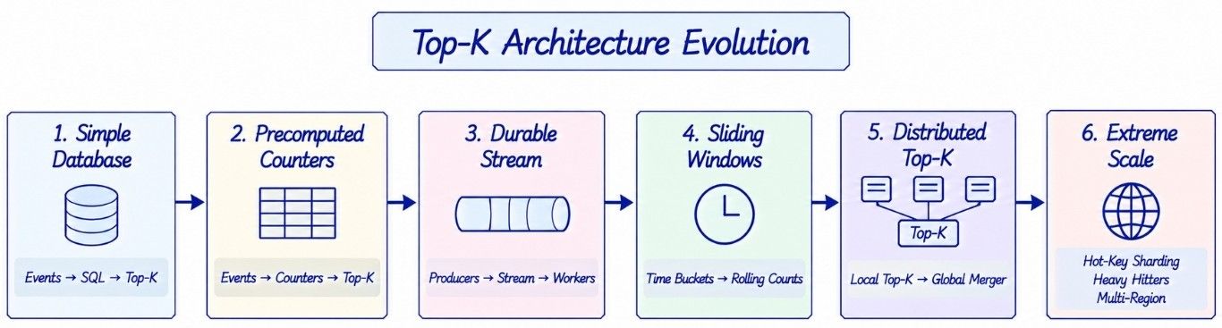
Lifetime counters are not enough for real-time trends. The system can add:

• Time buckets.

• Rolling window counts.

• Event-time processing.

• Late-event handling.

This allows the ranking to represent recent activity instead of lifetime popularity.

Distributed Top-K

When one worker cannot maintain the complete ranking, calculate Top-K across multiple partitions:

Partitioned Counts
       ↓
Local Top-K
       ↓
Global Top-K Merger
       ↓
Materialized Ranking
       ↓
Cache

When each logical item has one complete owner, only strong local candidates need to reach the global merger.

If an item is sharded across workers, its partial counts must first be combined before the final ranking.

Extreme Scale

At very large scale, additional techniques can solve specific bottlenecks:

• Hot-key sharding for highly popular items.

• Heavy-hitter algorithms for very high cardinality.

• Count-Min Sketch when exact counters use too much memory.

• Approximate candidate generation followed by exact reranking.

• Regional aggregation for global traffic.

• Multi-region processing and merging.

These techniques should be introduced only when simpler approaches no longer meet the required scale, freshness, accuracy, or cost targets.

Add complexity when it solves a real system bottleneck, not just because the technique exists.

Important Top-K Trending System Trade-Offs

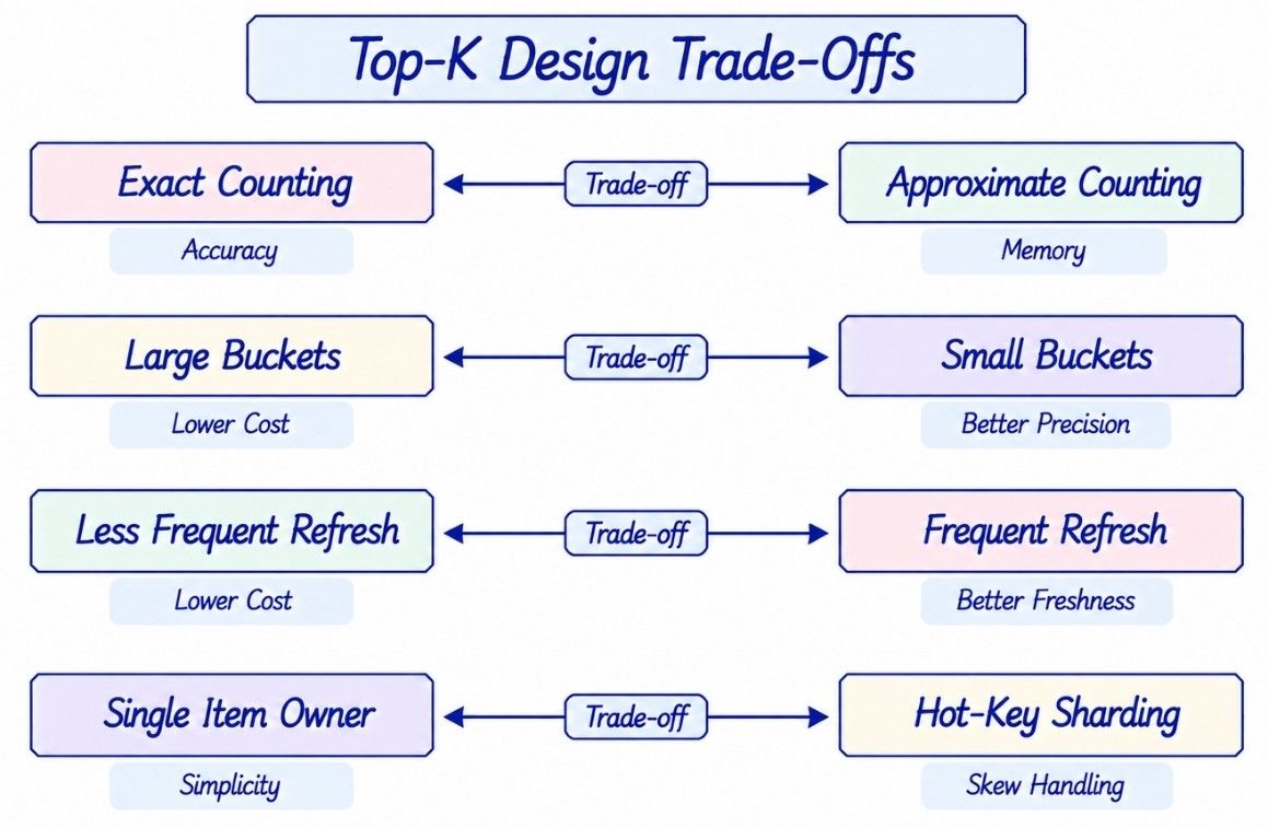
There is no single best Top-K architecture. The right choices depend on traffic, item cardinality, ranking accuracy, freshness, and cost.

The important interview skill is to explain why a trade-off fits the given requirements, rather than choosing the most complex option by default.

Common Top-K Trending System Design Mistakes

Common mistakes include:

• Not defining what trending means before designing the system.

• Scanning, grouping, and sorting raw events for every client request.

• Ignoring sliding-window expiration and allowing old activity to affect current trends.

• Keeping every raw event in processor memory instead of maintaining bounded aggregation state.

• Using processing time everywhere and ignoring event time and late events.

• Assuming partitioning by item_id cannot create hot partitions.

• Sharding a hot item but ranking its partial counts before reducing them into one logical count.

• Introducing Count-Min Sketch too early or assuming it directly returns Top-K item IDs.

• Precomputing every possible geography, category, and time-window combination.

• Calculating rankings synchronously when clients request them instead of serving materialized results.

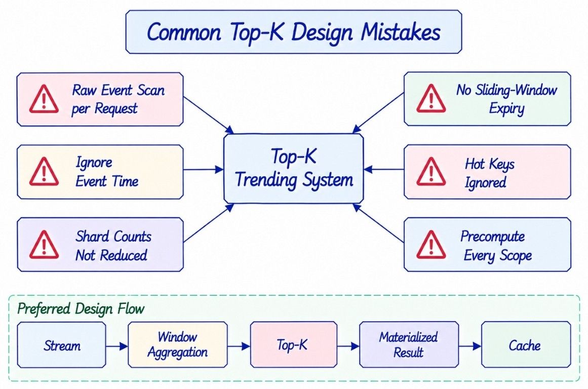
The core idea is to continuously aggregate recent activity, maintain Top-K rankings in the background, and serve small materialized results instead of rebuilding the ranking for every request.

Most Common Top-K Trending System Design Interview Questions

Q1. What is a Top-K system?

A Top-K system continuously identifies the K highest-scoring items from a large dataset or event stream, such as popular songs, videos, search queries, or hashtags.

Q2. What is the difference between Top-K and trending?

Top-K can mean highest overall popularity. Trending usually emphasizes recent activity, growth, or another time-sensitive score.

Q3. Why not query raw events for every request?

At high scale, each query could scan and group billions of events. Incremental aggregation makes the read path much faster.

Q4. How do you calculate Top-K efficiently?

Maintain item counts and use a min-heap of size K when selecting candidates. This reduces selection from roughly O(N log N) sorting to O(N log K).

Q5. How do you distribute Top-K computation?

Partition items across workers, calculate local Top-K candidates, and merge those candidates to produce the global ranking.

Q6. How do you support sliding windows?

Maintain fixed-size time buckets and a rolling total. Add new buckets and subtract expired buckets as the window moves.

Q7. Why not keep every timestamp in memory?

Bucketed aggregation uses much less state and makes sliding-window updates efficient.

Q8. How do you support multiple time windows?

Use reusable minute, hour, and day buckets or maintain selected independent windows based on query patterns.

Q9. How do you handle late events?

Use event-time processing with bounded lateness and watermarks so delayed events can update the correct recent bucket.

Q10. What happens if one hashtag becomes extremely popular?

It can create a hot partition. Split the item into sub-shards, calculate partial counts, and reduce them before Top-K calculation.

Q11. Why not always partition by item ID?

It provides simple ownership, but one viral item can overload the single partition responsible for it.

Q12. What is Count-Min Sketch?

Count-Min Sketch is a probabilistic frequency-estimation structure that uses bounded memory but may slightly overestimate counts because of hash collisions.

Q13. How do you get Top-K from Count-Min Sketch?

Use the sketch for frequency estimates and maintain a separate candidate heap or heavy-hitter structure containing item identities.

Q14. When should approximate Top-K be used?

Use it when item cardinality is extremely high, exact state is expensive, and small errors are acceptable.

Q15. How can you improve accuracy near the K boundary?

Generate a candidate set larger than K, calculate more accurate counts for those candidates, and rerank them.

Q16. How do you support country-specific trends?

Include geographic scope in events and maintain materialized rankings for selected countries or regions.

Q17. How do you prevent geographic cardinality explosion?

Precompute only important scopes and use a separate analytics system for rare arbitrary combinations.

Q18. How do you detect actual trends instead of existing popularity?

Compare recent activity with historical baselines or include growth, velocity, decay, and minimum-volume thresholds.

Q19. How do you prevent bots from dominating trends?

Use unique-user signals, rate limits, abuse detection, eligibility rules, and filtering or downweighting of suspicious activity.

Q20. How do you recover from processor failure?

Keep events in a durable stream, checkpoint processor state, reassign the partition, restore the checkpoint, and replay remaining events.

Q21. Why is eventual consistency acceptable?

Trending results usually tolerate a few seconds of staleness. Strong global coordination after every event would be much more expensive.

Q22. How do you handle duplicate events?

Use stable event IDs and idempotent or deduplicated processing when the required ranking accuracy justifies the additional state.

Q23. How do you scale reads?

Precompute small Top-K results and serve them through a cache instead of running ranking computation for every request.

Q24. How do you scale globally?

Perform regional ingestion and aggregation, then merge regional partial results or candidates into global rankings.

Q25. What metrics would you monitor?

Monitor event throughput, stream lag, oldest-event age, processing throughput, state size, hot partitions, ranking refresh latency, event-to-trend latency, cache hit rate, and ranking age.

Final Top-K Trending Architecture

The final architecture keeps expensive ranking computation away from the client request path.

                       USER ACTIVITY
                            |
                            v
                      EVENT PRODUCERS
                            |
                            v
                  PARTITIONED EVENT STREAM
                            |
          +-----------------+-----------------+
          |                 |                 |
          v                 v                 v
      Worker A          Worker B          Worker C
          |                 |                 |
     Time Buckets      Time Buckets      Time Buckets
          |                 |                 |
    Rolling Counts     Rolling Counts     Rolling Counts
          |                 |                 |
     Local Top-K        Local Top-K        Local Top-K
          \                 |                 /
           \                |                /
            +---------------+---------------+
                            |
                            v
                    GLOBAL TOP-K MERGER
                            |
                            v
                      TRENDING STORE
                            |
                            v
                          CACHE
                            |
                            v
                    TRENDING SERVICE
                            |
                            v
                          CLIENT

For extremely high cardinality:

Massive Event Stream
        ↓
Approximate Heavy-Hitter Detection
        ↓
Candidate Set
        ↓
Exact Reranking
        ↓
Final Top-K

For hot items:

Hot Item
   ↓
Shard Across Partitions
   ↓
Partial Counts
   ↓
Reduce by Item
   ↓
Top-K Pipeline

For recovery:

Event Stream
     |
     +------→ Checkpointed Stream Processing
     |
     +------→ Raw Event Archive
                    ↓
              Replay / Recompute

The central design principle is:

Do not repeatedly scan and sort the complete event history. Aggregate events incrementally into bounded time windows, calculate Top-K locally, merge strong candidates globally, and introduce approximate heavy-hitter techniques only when exact per-item state becomes too expensive.