Google Maps / Location Service

Designing a Google Maps-like location service is a popular system design interview problem because it combines geospatial search, map rendering, GPS location tracking, routing, traffic, caching, and massive read traffic.

A user may simply:

Open Map
   ↓
Search Place
   ↓
Select Destination
   ↓
Get Route

But these actions require several specialized systems.

A Google Maps-like platform needs to answer questions such as:

Where am I?
What places are near me?
Where is this address?
How do I get from A to B?
What is the fastest route?
How long will the journey take?
Which roads currently have traffic?

The key idea is that a map platform is not one giant database of latitude and longitude values. Different workloads need different data structures and services.

Scope: This article designs a conceptual Google Maps-like platform for system design interviews. It does not describe Google’s private production architecture.

Functional Requirements

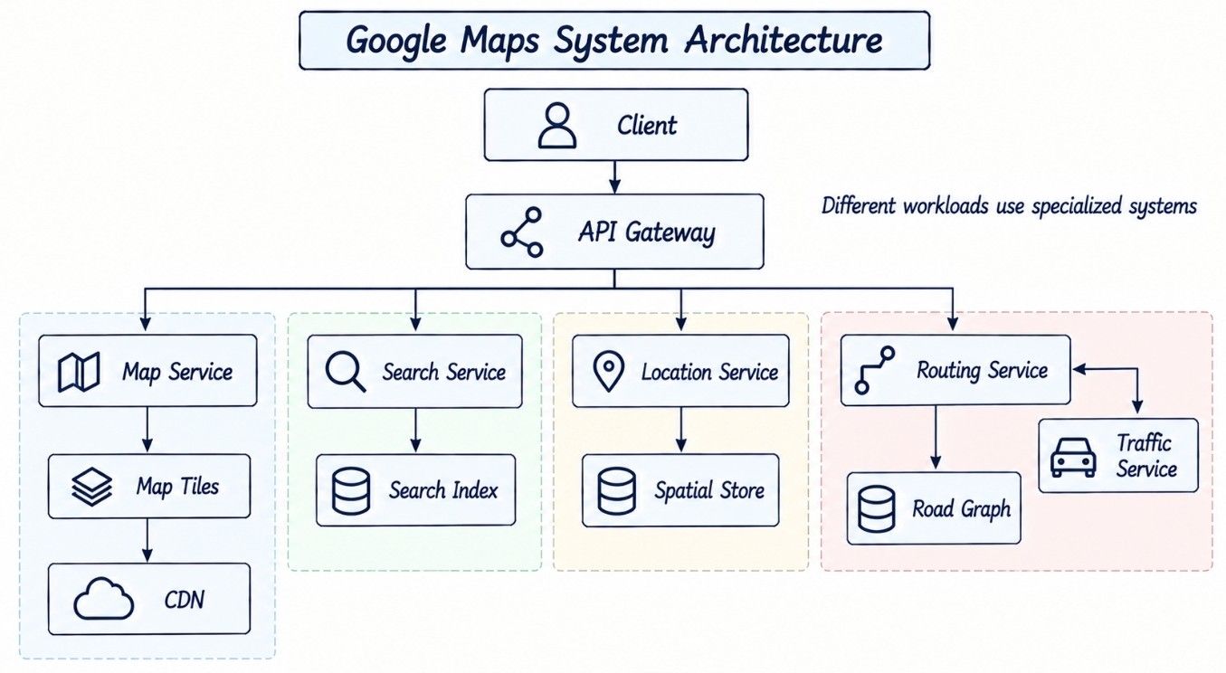
The system should support the core features users expect from a modern location platform.

• Display an interactive map.

• Show the user's current location.

• Search places and addresses.

• Perform geocoding and reverse geocoding.

• Find nearby places.

• Calculate routes between locations.

• Estimate travel time.

• Provide turn-by-turn navigation.

• Support traffic-aware routing.

Optional features include location sharing, geofencing, offline maps, public transit, walking/cycling routes, and multiple stops.

Non-Functional Requirements

A location service must handle global traffic while keeping map interactions and routing responsive.

• Low latency.

• High availability.

• High read throughput.

• Global scalability.

• Efficient spatial queries.

• Fresh traffic and location data.

• Horizontal scalability.

• Fault tolerance.

• Privacy and access control.

Different features need different consistency guarantees.

Map Tiles
→ aggressively cached

Place Search
→ eventual consistency

Traffic
→ freshness is important

Live Location
→ low latency + freshness

Road Closures
→ fast propagation

Scale Estimation

We use hypothetical interview numbers to understand the scale rather than claiming actual Google Maps traffic.

Assume:

This gives approximately:

Map Interactions
500M × 20
= 10B/day
≈ 116,000/sec average

Place Searches
500M × 5
= 2.5B/day
≈ 29,000/sec average

Route Requests
500M × 2
= 1B/day
≈ 11,600/sec average

Peak traffic can be several times higher, and one visible map may require multiple tile requests.

This immediately suggests:

Map rendering should rely heavily on CDN and caching instead of generating every map view dynamically.

High-Level Architecture

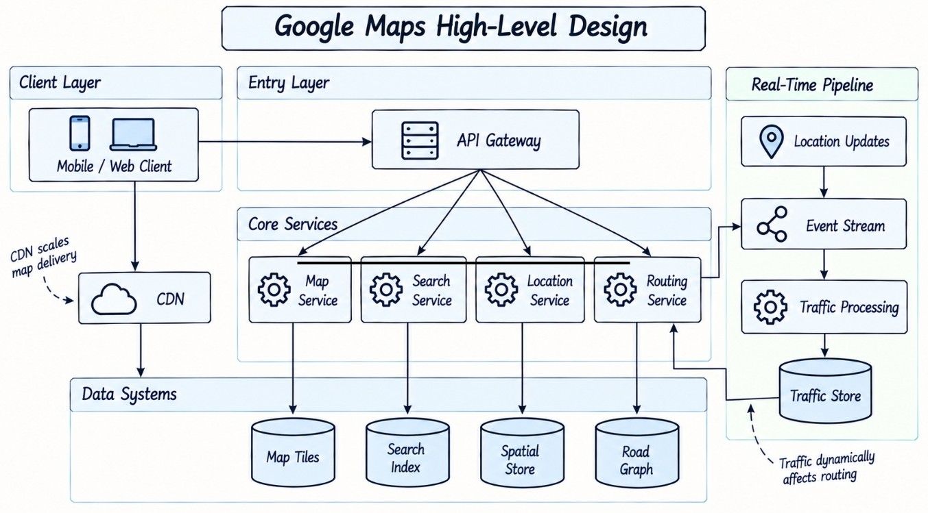
A Google Maps-like system contains specialized services for map delivery, search, location, routing, and traffic.

                         CLIENT
                           |
                           v
                      API Gateway
                           |
          +----------------+----------------+
          |                |                |
          v                v                v
     Map Service      Search Service   Location Service
          |                |                |
          v                v                v
      Tile Store       Search Index     Geo Store
          |
          v
         CDN

                       Routing Service
                            |
                    +-------+-------+
                    |               |
                    v               v
                Road Graph      Traffic Service
                                    |
                                    v
                              Traffic Pipeline

Additional services may include:

Geocoding
Reverse Geocoding
ETA
Navigation
Location Sharing
Geofencing

The important point is that these are different read and processing paths, not one large backend request.

Core Data Model

Different parts of the platform need different entities and access patterns.

Place
-----
place_id
name
latitude
longitude
category
address
metadata

RoadSegment
-----------
segment_id
start_node
end_node
distance
speed_limit
road_type
direction
restrictions

MapTile
-------
tile_id
zoom_level
x
y
version

TrafficObservation
------------------
road_segment_id
speed
timestamp

UserLocation
------------
user_id
latitude
longitude
accuracy
timestamp

Because these entities have very different workloads, using one database technology for everything is usually a poor design.

Latitude, Longitude, and Spatial Search

A geographic location is commonly represented using latitude and longitude.

{
  "latitude": 26.8467,
  "longitude": 80.9462
}

Storing coordinates is simple. The real challenge is efficiently finding nearby places among millions of locations.

User Location
     ↓
Millions of Places
     ↓
Find Nearby Places

Scanning every location or relying on simple latitude/longitude comparisons becomes inefficient at large scale.

To solve this efficiently, we need a geospatial index.

Geospatial Indexing

A geospatial index reduces the search space by dividing geographic areas into smaller cells.

+------+------+------+
| A1   | A2   | A3   |
+------+------+------+
| B1   | B2   | B3   |
+------+------+------+
| C1   | C2   | C3   |
+------+------+------+

Places can then be grouped by their spatial cell.

B2
 |
 +--> Restaurant
 +--> Hospital
 +--> ATM
 +--> Hotel

A nearby search becomes:

User Location
     ↓
Determine Spatial Cell
     ↓
Current + Neighboring Cells
     ↓
Candidate Places
     ↓
Exact Distance
     ↓
Filter + Rank
     ↓
Top Results

Instead of searching millions of places, the system searches only geographically relevant cells.

Geohash and Spatial Index Options

Geohash is one way to convert latitude and longitude into hierarchical geographic identifiers.

(latitude, longitude)
        ↓
     Geo Cell
        ↓
    "abc123..."

Higher precision represents a smaller geographic area.

Geohash is not the only spatial indexing approach.

A Quadtree can be useful when dense areas need finer subdivision than sparse regions.

Geohash Boundary Problem

Nearby locations can fall into different cells, especially near cell boundaries.

+-------------+-------------+
|          U  | R           |
|        User | Restaurant  |
+-------------+-------------+

Searching only the user's current cell could therefore miss nearby places.

Current Cell
     +
Neighboring Cells
     ↓
Candidate Places
     ↓
Exact Distance

So nearby search should usually consider the current cell plus relevant neighboring cells.

Nearby Search

Nearby search combines the user's query with their geographic location.

"coffee near me"

The request can be processed as:

Query + User Location
         ↓
Nearby Search Service
         ↓
Spatial Index
         ↓
Relevant Geo Cells
         ↓
Candidate Places
         ↓
Filter + Rank
         ↓
Top K Results

Filtering can consider category, distance, open status, availability, and user-selected filters, while ranking can consider relevance, popularity, quality, distance, and user context.

Geographical Distance vs Driving Distance

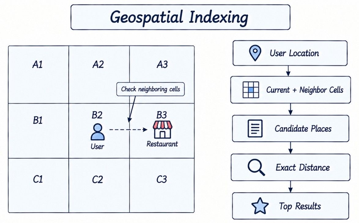
These three measurements represent different concepts in a location service.

Geographical Distance
        ≠
Driving Distance
        ≠
Travel Time

Spatial distance helps find nearby candidates, while the road network and traffic determine the actual route and travel time.

Place Search and Autocomplete

Place search combines text matching with geographic context to find relevant locations.

Example queries:

Starbucks
coffee near me
New Delhi Airport
221B Baker Street

A place-search index may contain:

Name
Aliases
Address
Category
Coordinates
Popularity
Language-specific Names
Metadata

The search flow is:

Query
  ↓
Normalization
  ↓
Candidate Retrieval
  ↓
Geographical Filtering
  ↓
Ranking
  ↓
Results

Ranking can consider text relevance, distance, popularity, category, open status, user context, and geographic importance.

Autocomplete

Autocomplete must return suggestions with very low latency while the user is still typing.

"New Del..."
      ↓
Autocomplete Service
      ↓
Prefix Index
      ↓
Candidate Places
      ↓
Location-Aware Ranking
      ↓
Suggestions

Popular prefixes and suggestions can be cached to reduce latency.

Geocoding and Reverse Geocoding

Geocoding and reverse geocoding convert between human-readable addresses and geographic coordinates.

Conceptually:

Geocoding

Address / Place
      ↓
Geocoding Service
      ↓
Latitude + Longitude

Reverse Geocoding

Latitude + Longitude
      ↓
Reverse Geocoding Service
      ↓
Road / Locality / Address

A global geocoding system must understand countries, cities, postal codes, streets, building numbers, landmarks, aliases, and regional address formats.

Map Rendering and Map Tiles

Generating an entire map image dynamically for every pan and zoom operation would be expensive.

Instead, divide the map into tiles.

+------+------+------+
| Tile | Tile | Tile |
+------+------+------+
| Tile | Tile | Tile |
+------+------+------+
| Tile | Tile | Tile |
+------+------+------+

A tile can be identified conceptually by:

zoom
x
y

For example:

/tiles/12/2341/1567

Low zoom levels cover large regions with less detail, while higher zoom levels cover smaller regions with greater detail.

The client downloads only the tiles required for the visible viewport.

Raster vs Vector Tiles

Raster and vector tiles differ mainly in what they store and where map rendering happens.

Vector tiles allow the client to dynamically render roads, labels, buildings, and other map features, making them well suited for interactive map applications.

CDN for Map Tiles

Map tiles are highly cacheable and are a strong use case for CDN delivery.

Client
  ↓
CDN
  |
  +── HIT → Return Tile
  |
  └── MISS
        ↓
     Tile Origin
        ↓
     Tile Store

This reduces latency, origin bandwidth, and central server load.

Popular geographic areas may achieve very high cache-hit rates.

Tile and Dataset Versioning

Roads, businesses, and map styles change over time.

Instead of unpredictably modifying cached tiles, use versioned assets.

/tiles/v42/zoom/x/y

When new map data is published:

v42 → v43

Clients gradually request the new version while old cached assets expire naturally.

Versioning also helps coordinate other derived datasets:

Map Dataset v101
      |
      +--> Tiles v101
      +--> Search Index v101
      +--> Road Graph v101
      +--> Geocoder v101

This improves cacheability, compatibility, rollback, and publication consistency.

Road Network as a Graph

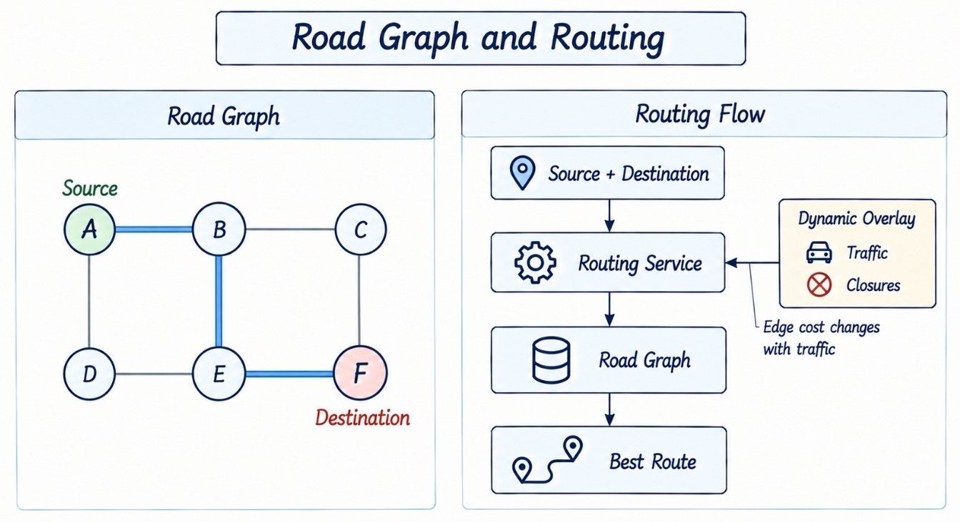
Routing requires a different data model from nearby search.

Represent roads as a graph.

A ----- B ----- C
|       |       |
|       |       |
D ----- E ----- F

Intersections become nodes, while road segments become edges.

Each edge can contain:

Distance
Expected Travel Time
Speed
Road Type
Direction
Turn Restrictions
Tolls
Access Restrictions

Routing then becomes a weighted graph-search problem.

Route Calculation

Suppose:

Start = A
Destination = F

For shortest-distance routing:

edge weight = distance

For fastest routing:

edge weight = estimated travel time

Conceptual algorithms include Dijkstra's algorithm and A*.

A* uses a heuristic to guide exploration toward the destination and can avoid exploring many irrelevant nodes.

Scaling Routing Beyond Basic Graph Search

Running a basic graph search across the entire global road network for every route request would be too expensive.

Large-scale routing reduces the search space using techniques such as:

• Graph partitioning — divide the road network into regions.

• Hierarchical routing — prefer higher-level roads for long-distance travel.

• Bidirectional search — search from both source and destination.

• Precomputed shortcuts — skip unnecessary intermediate road segments.

• Route preprocessing — prepare reusable routing data in advance.

For long-distance routes:

Local Roads
    ↓
Major Roads / Highways
    ↓
Local Roads Near Destination

The goal is to explore only the relevant part of the road graph instead of every possible road segment.

Route API

The Routing Service accepts an origin, destination, and travel mode and returns the calculated route.

POST /v1/routes

{
  "origin": {
    "lat": 26.8467,
    "lng": 80.9462
  },
  "destination": {
    "lat": 28.6139,
    "lng": 77.2090
  },
  "mode": "DRIVING"
}

A response may contain:

{
  "route_id": "R123",
  "distance_meters": 500000,
  "duration_seconds": 25000,
  "polyline": "...",
  "steps": []
}

The service may also return multiple candidate routes, allowing the client to compare alternatives based on distance, ETA, traffic, or road conditions.

Base Road Graph and Dynamic Overlay

Routing should separate relatively stable road data from frequently changing real-time conditions.

Base Road Graph
       +
Dynamic Overlay
       ↓
Routing Service
       ↓
Best Route

This separation allows traffic and temporary road conditions to affect routing without rebuilding the entire road graph.

Map Matching

GPS coordinates are noisy and may not fall exactly on a road, so the system must determine the most likely road segment.

       GPS Point
          *
          |
Road ----------------

Map matching converts the raw GPS observation into a likely road position.

GPS Observation
      ↓
Map Matching
      ↓
Likely Road Segment

This is important for navigation, route progress, rerouting, and traffic estimation.

Location Service

The Location Service handles high-frequency location updates from user devices.

Mobile Device
     ↓
Location Gateway
     ↓
Location Service
     |
     +--> Latest Location Store
     |
     +--> Event Stream

A location update may contain:

{
  "entity_id": "U123",
  "latitude": 26.8467,
  "longitude": 80.9462,
  "accuracy_meters": 8,
  "timestamp": 1789630000
}

The Latest Location Store keeps the most recent position, while the Event Stream allows downstream systems such as traffic processing and navigation to consume location updates asynchronously.

Not every raw GPS update needs to be stored permanently; current location and historical analytics have different storage and retention requirements.

Location Freshness and Update Frequency

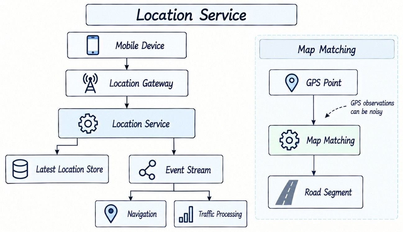
A location is meaningful only when the system also knows when it was recorded and how accurate it is.

Store at least:

coordinates
timestamp
accuracy

Update frequency should be adaptive. A moving user during navigation may send frequent updates, while a stationary device can update less often to save battery and bandwidth.

Factors include movement, speed, battery, network conditions, GPS accuracy, and application state.

Location Sharing

Live location sharing requires real-time delivery along with strict authorization and expiration controls.

Alice Phone
     ↓
Location Service
     ↓
Sharing Service
     ↓
Real-Time Gateway
     ↓
Bob Phone

A sharing record may contain:

share_id
owner_user_id
viewer_user_id
expires_at
permissions

The sharing lifecycle should be explicit:

ACTIVE → EXPIRED
ACTIVE → REVOKED

For active sessions, WebSockets or another streaming mechanism can efficiently deliver updates. The Sharing Service must verify that the viewer is authorized before exposing location data.

Geofencing

A geofence represents a geographic region where the system detects events such as ENTER and EXIT.

Checking every location update against every geofence would be too expensive at scale.

Location Update
      ↓
Spatial Cell
      ↓
Candidate Geofences
      ↓
Exact Geometry Check
      ↓
ENTER / EXIT Event

The spatial index first finds nearby candidate geofences, and the system performs the more expensive geometry check only on those candidates.

Spatial indexing prevents every location update from being compared with every geofence.

Traffic Processing

Traffic is dynamic and should not be treated as permanent map data.

A road segment might normally support:

60 km/h

but currently average:

15 km/h

Traffic data can conceptually come from aggregated device observations, road sensors, public road data, incidents, and historical patterns.

A scalable processing pipeline looks like:

Location / Traffic Observations
             ↓
         Event Stream
             ↓
       Stream Processing
             ↓
         Map Matching
             ↓
     Traffic Aggregation
             ↓
        Traffic Store
             ↓
      Routing / ETA

Traffic is therefore a natural stream-processing workload.

Traffic Aggregation and Freshness

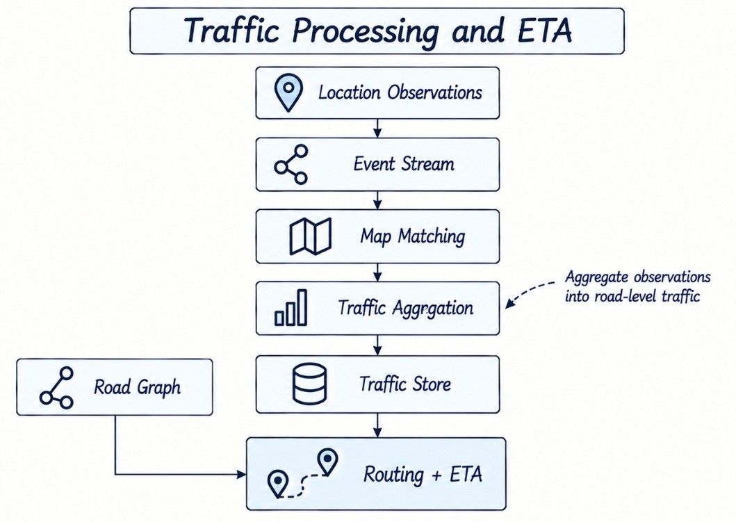
Individual observations should usually be aggregated into road-level estimates.

Vehicle Observations
        +
Historical Data
        ↓
Road Segment
        ↓
Estimated Speed

Aggregation reduces noise and helps protect individual privacy.

Traffic data also needs freshness controls.

timestamp
TTL
freshness weighting

If live traffic becomes unavailable, routing can fall back to historical traffic, typical travel times, or speed limits instead of failing completely.

ETA Service

Routing answers:

Which path should I take?

ETA answers:

How long will it take?

ETA may depend on:

Route Segments
Current Traffic
Historical Traffic
Time of Day
Day of Week
Road Type
Turn Delays
Incidents

Conceptually:

Route
  +
Traffic
  +
Historical Model
      ↓
ETA Service
      ↓
Estimated Arrival Time

Two routes with equal physical distance can have very different ETAs because of highways, traffic lights, congestion, and road restrictions.

Turn-by-Turn Navigation and Rerouting

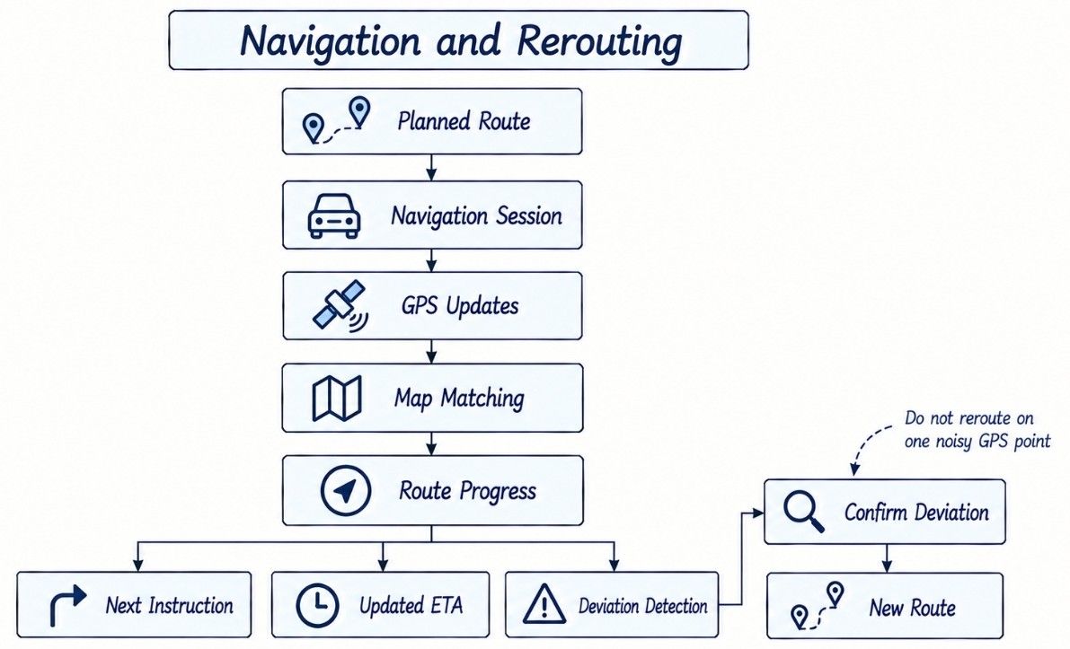
Turn-by-turn navigation continuously compares the planned route with the user's latest location.

Route
  ↓
Navigation Session
  ↓
GPS Updates
  ↓
Map Matching
  ↓
Route Progress
  |
  +--> Next Instruction
  +--> Updated ETA
  +--> Deviation Detection

If the user moves away from the planned route:

Route Deviation
      ↓
Confirm Deviation
      ↓
Rerouting
      ↓
New Route + ETA

The system should not reroute on every noisy GPS point. It should use GPS accuracy, map matching, multiple observations, and a deviation threshold before confirming that the user is off-route.

Map Data Update Pipeline

Map data changes continuously as roads, businesses, street names, and restrictions are added or updated.

Map Data Sources
      ↓
Validation
      ↓
Normalization
      ↓
Map Database
      |
      +--> Tile Generation
      +--> Search Index
      +--> Routing Graph
      +--> Geocoding Index

These derived datasets can be rebuilt and published independently.

Because updating every system atomically is difficult, dataset versioning and coordinated publication help keep tiles, search, routing, and geocoding data reasonably consistent.

Map Dataset v101
      |
      +--> Tiles v101
      +--> Search Index v101
      +--> Road Graph v101
      +--> Geocoder v101

Build and validate the new dataset first, then publish the new version instead of partially updating live map data.

Offline Maps

Users may download a geographic region for offline use.

Selected Region
      ↓
Offline Package Service
      ↓
Map Data
+ Search Data
+ Routing Data
      ↓
Mobile Device

Challenges include package size, storage, updates, version compatibility, and the lack of fresh traffic information.

Offline routing may use a reduced local road graph.

Geospatial Partitioning

Geography is a natural partitioning dimension.

World
  ↓
Region
  ↓
Spatial Cell

Spatially related data can therefore be kept close together.

However, traffic density is highly uneven.

Airport
Stadium
City Center
Popular Tourist Area

may receive far more traffic than rural cells.

Mitigations include adaptive subdivision, virtual shards, caching, replicas, and load-aware routing.

Cross-Partition Queries

Nearby searches close to a partition boundary may require multiple shards.

Shard A | Shard B
        |
       User

The query coordinator can:

Relevant Shards
      ↓
Parallel Queries
      ↓
Merge Candidates
      ↓
Rank

The system should query only relevant neighboring partitions rather than broadcasting globally.

Multi-Region Architecture

A global location platform benefits from regional deployments.

                   Global Router
                        |
          +-------------+-------------+
          |             |             |
          v             v             v
       Region A      Region B      Region C
          |             |             |
       Search         Search         Search
       Routing        Routing        Routing
       Location       Location       Location

Base map data, place information, and road graphs can be replicated regionally.

Dynamic workloads such as current traffic, navigation sessions, and live location updates are naturally more regional.

This reduces latency and improves fault isolation.

Caching Strategy

Different data requires different caching policies.

Good candidates include:

• Map tiles.

• Popular place searches.

• Autocomplete prefixes.

• Place details.

• Geocoding results.

• Static road information.

Dynamic data requires more care:

Live Traffic
Live Location
Temporary Closures

These need short TTLs, freshness checks, or event-driven invalidation.

A popular tile expiring simultaneously across caches can also cause a cache stampede.

Mitigations include request coalescing, background refresh, jittered expiration, stale-while-revalidate, and multi-layer caching.

High-Volume Location Ingestion

Suppose 10 million active navigation sessions each send one location update every five seconds.

10M / 5
= 2 million updates/sec

This workload is fundamentally different from ordinary profile updates.

Use:

Location Gateway
      ↓
Durable Event Stream
      |
      +--> Traffic Processing
      +--> Navigation
      +--> Analytics
      +--> Safety / Quality

The event stream prevents the ingestion service from synchronously calling every downstream consumer.

It also provides buffering when consumers temporarily slow down.

Backpressure

If a downstream traffic processor slows down, it should not block location ingestion.

Location Ingestion
      ↓
Durable Buffer
      ↓
Independent Consumers

Monitor queue lag, oldest event age, processing throughput, and dropped or expired observations.

Not every location event needs identical priority or retention.

Location Privacy and Abuse Protection

Location information can reveal sensitive patterns about a user's movements, so the architecture should minimize unnecessary collection and exposure.

Important controls include:

• Authentication and authorization.

• Encryption in transit and at rest.

• Data minimization.

• Retention controls.

• Access auditing.

• Explicit location-sharing permissions.

• Rate limits and API quotas.

• Anomaly detection.

• Protection against fake GPS and traffic manipulation.

Traffic consumers should normally receive aggregated road-level information rather than individual user trajectories.

Failure Handling and Graceful Degradation

A location platform contains many independent capabilities, so one failure should not unnecessarily break the entire product.

Graceful degradation is especially important for navigation.

Consistency Requirements

Different map workflows require different consistency models.

The goal is not strong consistency everywhere.

The goal is the correct guarantee for each workflow.

Observability

Monitor each major subsystem separately.

Also measure user-facing end-to-end latency rather than only individual service latency.

Complete Map Rendering Flow

The client requests only the map tiles needed for its current viewport.

User Opens Map
      ↓
Determine Viewport
      ↓
Calculate Tile IDs
      ↓
CDN
  +---+---+
 HIT     MISS
  |        |
  |        v
  |    Tile Origin
  |        ↓
  |    Tile Store
  ↓
Return Tiles
      ↓
Client Renders Map

As the user pans or zooms, additional tiles are fetched.

Complete Nearby Search Flow

Nearby search combines textual intent with spatial indexing.

"coffee near me"
       ↓
Search Service
       ↓
Query / Category
       +
User Location
       ↓
Spatial Index
       ↓
Current + Neighbor Cells
       ↓
Candidate Places
       ↓
Filter + Distance + Rank
       ↓
Top K Results

Complete Routing Flow

Routing combines a mostly stable road graph with dynamic conditions.

Origin + Destination
        ↓
Routing Service
        ↓
Snap to Road Graph
        ↓
Graph Search
   +----+----+
   |         |
   v         v
Base Graph  Dynamic Overlay
             |
        Traffic / Closures
             ↓
      Candidate Routes
             ↓
          ETA
             ↓
       Rank Routes
             ↓
Route + Steps + ETA

Complete Navigation Flow

Navigation continuously combines the planned route with fresh device location.

Route
  ↓
Navigation Session
  ↓
GPS Updates
  ↓
Map Matching
  ↓
Route Progress
  |
  +--> Instructions
  +--> ETA Updates
  +--> Traffic Changes
  +--> Deviation Detection
              ↓
           Reroute

This is the central real-time navigation flow.

High-Level Design vs Low-Level Design

HLD focuses on distributed architecture and scale, while LLD focuses on domain objects and internal behavior.

For a Google Maps system design interview, start with HLD and move to class-level design only when required.

Architecture Evolution

A Google Maps-like architecture should grow as requirements and traffic increase.

Starting simple and introducing complexity only when a bottleneck requires it is more convincing than immediately naming many distributed technologies.

Key Trade-Offs

Every major subsystem involves a different trade-off.

• Geo cell size: smaller cells reduce candidates but increase index/partition complexity; larger cells are simpler but return more candidates.

• Tile freshness vs cacheability: long-lived tiles improve CDN efficiency but may become stale; versioning helps balance both.

• Routing accuracy vs latency: additional dynamic signals may improve route quality but increase computation.

• Location freshness vs battery: frequent GPS updates improve navigation but consume more battery and bandwidth.

• Precomputation vs flexibility: precomputed routing structures improve latency, while dynamic overlays handle traffic and temporary changes.

Most Asked Google Maps System Design Interview Questions

These questions cover the concepts most likely to require deeper explanation during a location-service system design interview.

Q1. How would you design Google Maps?

Separate the platform into map delivery, place search, geospatial indexing, geocoding, routing, traffic, ETA, and location services.

Serve cacheable map assets through a CDN and use specialized spatial and graph structures for geographic queries and routing.

Q2. How do you find nearby places?

Convert the user's coordinates into a spatial cell, search the current and neighboring cells, retrieve candidates, calculate actual distance, and rank the results.

Q3. Why do we need a geospatial index?

Without one, nearby searches may scan enormous datasets. Spatial indexing restricts queries to geographically relevant regions.

Q4. What is geohashing?

Geohashing converts coordinates into hierarchical geographic identifiers that group locations into spatial cells.

Q5. What is the geohash boundary problem?

Two nearby locations can fall into different cells. Search neighboring cells as well and calculate exact distance afterward.

Q6. Geohash vs Quadtree?

The correct choice depends on query patterns, density, and operational requirements.

Q7. How do you render maps efficiently?

Divide the map into tiles and distribute them through a CDN. The client downloads only tiles needed for its current viewport and zoom level.

Q8. What are vector tiles?

Vector tiles contain map geometry and features rather than pre-rendered images. The client renders them, allowing flexible styling and smoother zooming and rotation.

Q9. How do you calculate routes?

Represent roads as a weighted graph and use algorithms such as A*, combined with graph partitioning, hierarchy, preprocessing, and dynamic traffic data.

Q10. Why is naive Dijkstra not enough globally?

Running full graph exploration over a massive road network for every route request is too expensive.

Large-scale routing reduces the search space using hierarchy, heuristics, partitioning, bidirectional search, or precomputed shortcuts.

Q11. How do you calculate ETA?

Combine route segments with current traffic, historical traffic, road properties, time context, turn delays, and incidents.

Q12. How do you incorporate traffic?

Map observations to road segments, aggregate them into current speed estimates, and use those estimates as dynamic routing costs.

Q13. What if live traffic is unavailable?

Fall back to historical traffic, typical travel times, or speed-limit-based estimates instead of making routing unavailable.

Q14. What is map matching?

Map matching converts noisy GPS observations into the most likely road segment or route position.

Q15. How do you detect route deviation?

Compare map-matched positions against the planned route over multiple observations. Reroute only when deviation confidence passes a threshold.

Q16. How do you design location sharing?

Store explicit permissions and expiration, ingest fresh owner locations, and deliver authorized updates through a real-time channel.

Q17. How do you design geofencing?

Spatially index geofences, retrieve nearby candidates for each location update, and perform exact geometry tests only on those candidates.

Q18. How do you partition geospatial data?

Partition primarily by geographic regions or hierarchical cells, while supporting neighboring-cell queries and adaptive subdivision.

Q19. How do you handle hot geographic regions?

Subdivide dense cells, use virtual shards or replicas, cache read-heavy data, and distribute processing rather than assigning the entire hot area to one fixed shard.

Q20. How do you handle map updates?

Validate and normalize source data, update the map database, rebuild derived datasets, and publish versioned tiles, indexes, geocoding data, and road graphs.

Q21. Why use versioned map datasets?

Versioning enables immutable caching, coordinated publication, compatibility checks, rollback, and cleaner transitions between map datasets.

Q22. How would you support offline maps?

Generate regional packages containing the map data and enough local search and routing information to support the required offline features.

Q23. How do you process millions of GPS updates?

Use a horizontally scalable ingestion layer, durable event stream, appropriate partitioning, and independent downstream consumers for traffic, navigation, and analytics.

Q24. What can be eventually consistent?

Place search, many map updates, traffic aggregates, and cached map assets can tolerate bounded staleness depending on the feature.

Authorization and safety-critical routing changes require stronger correctness or faster propagation.

Q25. What should you monitor?

Monitor tile/CDN performance, search latency, route latency, ETA accuracy, location freshness, traffic processing lag, hot partitions, rerouting frequency, and regional availability.

Common Mistakes

Avoid these common mistakes when designing a Google Maps-like system:

• Storing latitude and longitude without explaining spatial indexing.

• Searching only the current geospatial cell and ignoring neighboring cells.

• Treating straight-line distance as driving distance or ETA.

• Running naive graph traversal over the entire global road network.

• Generating every map view dynamically instead of using tiles and CDN.

• Storing every GPS update in the main transactional database.

• Rerouting after every noisy GPS observation.

• Treating traffic and temporary closures as permanent road data.

• Ignoring hot geographic partitions and map-data versioning.

• Starting with technology names instead of explaining the underlying problems.

Final Google Maps / Location Service Architecture

The final architecture separates static map delivery, geographic search, routing, and high-volume real-time traffic processing.

                           CLIENT
                              |
                    +---------+---------+
                    |                   |
                    v                   v
                API Gateway            CDN
                    |                   |
          +---------+---------+         v
          |         |         |     Map Tiles
          v         v         v
       Search    Location   Routing
       Service   Service   Service
          |         |         |
          v         v         v
       Search    Spatial   Road Graph
        Index     Store        |
                               +
                               |
                         Traffic Overlay
                               |
                               v
                          Route + ETA

MAP DATA PIPELINE

Raw / Validated Map Data
          |
          v
      Map Database
          |
    +-----+------+---------+-----------+
    |            |         |           |
    v            v         v           v
Tile Build    Search    Geocoder   Road Graph
    |          Index      Index      Builder
    v
Object Storage
    |
    v
   CDN

REAL-TIME TRAFFIC

Location Observations
         |
         v
   Ingestion Layer
         |
         v
     Event Stream
         |
         v
  Stream Processing
         |
         v
    Map Matching
         |
         v
Traffic Aggregation
         |
         v
   Traffic Store
         |
         v
    Routing / ETA

The central design principle is:

Use spatial indexes to reduce geographic search space, graph-based systems for routing, CDN-backed tiles for map delivery, and a separate real-time pipeline for dynamic location and traffic data.

Once these workloads are separated, the overall Google Maps System Design becomes much easier to scale, reason about, and explain in an interview.